E-Commerce Linear Regression Analysis

Author

Kushagra Shukla

1 Github Repository:

GitHub Repository

2 E-Commerce Linear Regression Analysis

This document presents the analysis of an e-commerce dataset using various statistical methods, including simple and multiple linear regression, feature engineering, and customer segmentation through K-means clustering.

2.1 1. Import Data and Basic Exploration

We begin by loading the dataset and performing a basic exploration.

ecomdata <- read.csv("./data/ecomdata")
str(ecomdata)
'data.frame':   500 obs. of  8 variables:
 $ Email               : chr  "mstephenson@fernandez.com" "hduke@hotmail.com" "pallen@yahoo.com" "riverarebecca@gmail.com" ...
 $ Address             : chr  "835 Frank Tunnel\nWrightmouth, MI 82180-9605" "4547 Archer Common\nDiazchester, CA 06566-8576" "24645 Valerie Unions Suite 582\nCobbborough, DC 99414-7564" "1414 David Throughway\nPort Jason, OH 22070-1220" ...
 $ Avatar              : chr  "Violet" "DarkGreen" "Bisque" "SaddleBrown" ...
 $ Avg..Session.Length : num  34.5 31.9 33 34.3 33.3 ...
 $ Time.on.App         : num  12.7 11.1 11.3 13.7 12.8 ...
 $ Time.on.Website     : num  39.6 37.3 37.1 36.7 37.5 ...
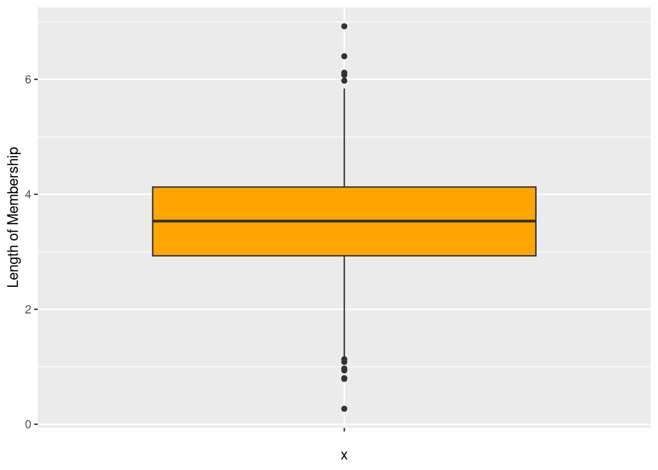
 $ Length.of.Membership: num  4.08 2.66 4.1 3.12 4.45 ...
 $ Yearly.Amount.Spent : num  588 392 488 582 599 ...
summary(ecomdata)
    Email             Address             Avatar          Avg..Session.Length
 Length:500         Length:500         Length:500         Min.   :29.53      
 Class :character   Class :character   Class :character   1st Qu.:32.34      
 Mode  :character   Mode  :character   Mode  :character   Median :33.08      
                                                          Mean   :33.05      
                                                          3rd Qu.:33.71      
                                                          Max.   :36.14      
  Time.on.App     Time.on.Website Length.of.Membership Yearly.Amount.Spent
 Min.   : 8.508   Min.   :33.91   Min.   :0.2699       Min.   :256.7      
 1st Qu.:11.388   1st Qu.:36.35   1st Qu.:2.9304       1st Qu.:445.0      
 Median :11.983   Median :37.07   Median :3.5340       Median :498.9      
 Mean   :12.052   Mean   :37.06   Mean   :3.5335       Mean   :499.3      
 3rd Qu.:12.754   3rd Qu.:37.72   3rd Qu.:4.1265       3rd Qu.:549.3      
 Max.   :15.127   Max.   :40.01   Max.   :6.9227       Max.   :765.5      

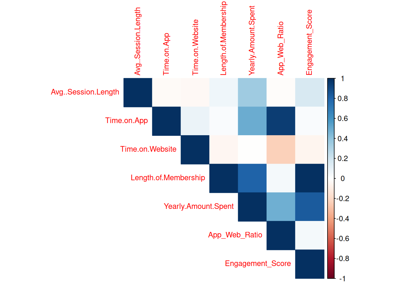
2.2 2. Visualization and Correlation Analysis

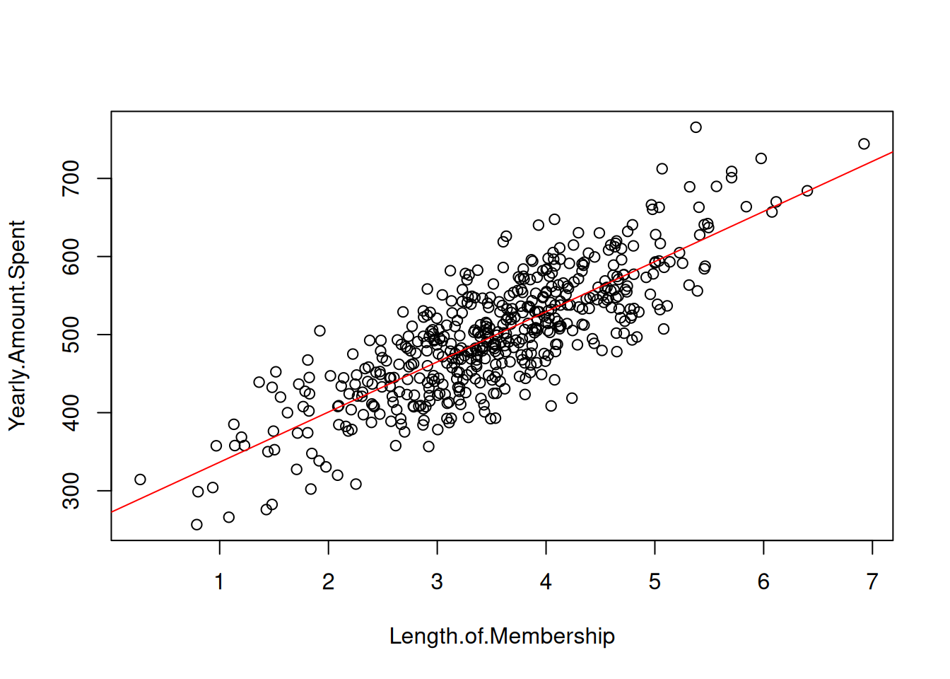
2.2.1 2.1 Scatter Plots

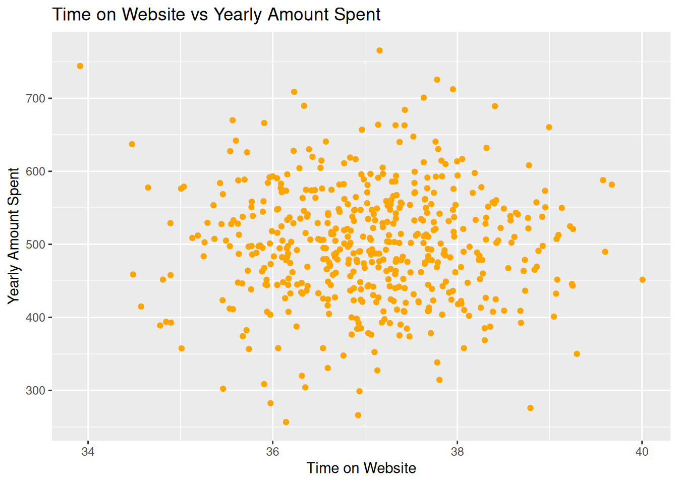
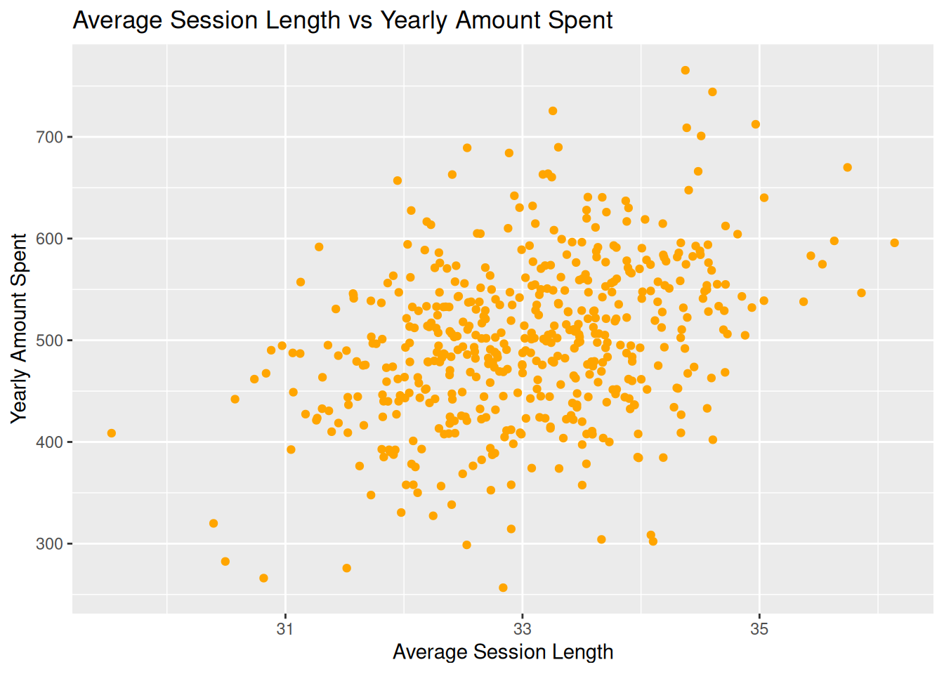
The following scatter plots show the relationship between various variables:

Time on Website vs Yearly Amount Spent

library(ggplot2)
ggplot(ecomdata, aes(x = Time.on.Website, y = Yearly.Amount.Spent)) + 
  geom_point(colour = "orange") + 
  ggtitle("Time on Website vs Yearly Amount Spent") + 
  xlab("Time on Website") +
  ylab("Yearly Amount Spent")

Average Session Length vs Yearly Amount Spent

ggplot(ecomdata, aes(x = Avg..Session.Length, y = Yearly.Amount.Spent)) + 
  geom_point(colour = "orange") +
  ggtitle("Average Session Length vs Yearly Amount Spent") + 
  xlab("Average Session Length") +
  ylab("Yearly Amount Spent")

2.2.2 2.2 Pairplot

pairs(ecomdata[c("Avg..Session.Length", "Time.on.App", "Time.on.Website", 
                 "Length.of.Membership", "Yearly.Amount.Spent")],
      col = "orange", pch = 16,
      labels = c("Avg Session Length", "Time on App", "Time on Website",
                 "Length of Membership", "Yearly Spent"),
      main = "Pairplot of Variables")

2.2.3 2.3 Histogram and Boxplot of Length of Membership

Histogram

ggplot(ecomdata, aes(x = Length.of.Membership)) + 
  geom_histogram(color = "white", fill = "orange", binwidth = 0.5)

Boxplot

ggplot(ecomdata, aes(x = "", y = Length.of.Membership)) + 
  geom_boxplot(fill = "orange") +
  ylab("Length of Membership")

2.3 3. Simple Linear Regression

We fit a simple linear regression model to predict Yearly Amount Spent based on Length of Membership.

lm.fit1 <- lm(Yearly.Amount.Spent ~ Length.of.Membership, data = ecomdata)
summary(lm.fit1)

Call:
lm(formula = Yearly.Amount.Spent ~ Length.of.Membership, data = ecomdata)

Residuals:
     Min       1Q   Median       3Q      Max 
-125.975  -29.032   -0.494   33.033  147.777 

Coefficients:
                     Estimate Std. Error t value Pr(>|t|)    
(Intercept)           272.400      7.675   35.49   <2e-16 ***
Length.of.Membership   64.219      2.090   30.72   <2e-16 ***
---
Signif. codes:  0 '***' 0.001 '**' 0.01 '*' 0.05 '.' 0.1 ' ' 1

Residual standard error: 46.66 on 498 degrees of freedom
Multiple R-squared:  0.6546,    Adjusted R-squared:  0.6539 
F-statistic: 943.9 on 1 and 498 DF,  p-value: < 2.2e-16

Regression Line

plot(Yearly.Amount.Spent ~ Length.of.Membership, data = ecomdata)
abline(lm.fit1, col = "red")

2.3.1 3.1 Residual Diagnostics

qqnorm(residuals(lm.fit1)); qqline(residuals(lm.fit1), col = "red")

shapiro.test(residuals(lm.fit1))

    Shapiro-Wilk normality test

data:  residuals(lm.fit1)
W = 0.99756, p-value = 0.6837

2.4 4. Train-Test Split and Model Evaluation (Simple Linear)

set.seed(1)
train_idx <- sample(1:nrow(ecomdata), 0.8 * nrow(ecomdata))
train <- ecomdata[train_idx, ]
test <- ecomdata[-train_idx, ]

lm.fit0.8 <- lm(Yearly.Amount.Spent ~ Length.of.Membership, data = train)
summary(lm.fit0.8)

Call:
lm(formula = Yearly.Amount.Spent ~ Length.of.Membership, data = train)

Residuals:
     Min       1Q   Median       3Q      Max 
-124.810  -29.274   -2.219   31.482  149.107 

Coefficients:
                     Estimate Std. Error t value Pr(>|t|)    
(Intercept)           271.853      8.691   31.28   <2e-16 ***
Length.of.Membership   64.073      2.355   27.21   <2e-16 ***
---
Signif. codes:  0 '***' 0.001 '**' 0.01 '*' 0.05 '.' 0.1 ' ' 1

Residual standard error: 47.14 on 398 degrees of freedom
Multiple R-squared:  0.6503,    Adjusted R-squared:  0.6494 
F-statistic: 740.2 on 1 and 398 DF,  p-value: < 2.2e-16
prediction0.8 <- predict(lm.fit0.8, newdata = test)
err0.8 <- prediction0.8 - test$Yearly.Amount.Spent
rmse <- sqrt(mean(err0.8^2))
mape <- mean(abs(err0.8 / test$Yearly.Amount.Spent))

c(RMSE = rmse, MAPE = mape, R2 = summary(lm.fit0.8)$r.squared)
       RMSE        MAPE          R2 
44.78105782  0.07692126  0.65032683 

2.5 5. Multiple Linear Regression

multi.lm.fit <- lm(Yearly.Amount.Spent ~ Avg..Session.Length + 
                     Time.on.App + Time.on.Website + 
                     Length.of.Membership, data = ecomdata)
summary(multi.lm.fit)

Call:
lm(formula = Yearly.Amount.Spent ~ Avg..Session.Length + Time.on.App + 
    Time.on.Website + Length.of.Membership, data = ecomdata)

Residuals:
     Min       1Q   Median       3Q      Max 
-30.4059  -6.2191  -0.1364   6.6048  30.3085 

Coefficients:
                       Estimate Std. Error t value Pr(>|t|)    
(Intercept)          -1051.5943    22.9925 -45.736   <2e-16 ***
Avg..Session.Length     25.7343     0.4510  57.057   <2e-16 ***
Time.on.App             38.7092     0.4510  85.828   <2e-16 ***
Time.on.Website          0.4367     0.4441   0.983    0.326    
Length.of.Membership    61.5773     0.4483 137.346   <2e-16 ***
---
Signif. codes:  0 '***' 0.001 '**' 0.01 '*' 0.05 '.' 0.1 ' ' 1

Residual standard error: 9.973 on 495 degrees of freedom
Multiple R-squared:  0.9843,    Adjusted R-squared:  0.9842 
F-statistic:  7766 on 4 and 495 DF,  p-value: < 2.2e-16

2.6 6. Feature Engineering and Correlation Matrix

ecomdata$App_Web_Ratio <- ecomdata$Time.on.App / (ecomdata$Time.on.Website + 1)
ecomdata$Engagement_Score <- ecomdata$Avg..Session.Length * ecomdata$Length.of.Membership

library(corrplot)
corrplot 0.95 loaded
num_data <- ecomdata[, sapply(ecomdata, is.numeric)]
cor_matrix <- cor(num_data, use = "complete.obs")
corrplot(cor_matrix, method = "color", type = "upper", tl.cex = 0.8)

2.7 7. Customer Segmentation: K-means Clustering

set.seed(2)
kmeans_result <- kmeans(ecomdata[, c("Avg..Session.Length", "Time.on.App", 
                                     "Time.on.Website", "Length.of.Membership")], 
                        centers = 3, nstart = 20)

ecomdata$Cluster <- as.factor(kmeans_result$cluster)

ggplot(ecomdata, aes(x = Avg..Session.Length, y = Time.on.App, color = Cluster)) + 
  geom_point() + 
  ggtitle("Customer Segmentation using K-means Clustering") +
  xlab("Avg. Session Length") + 
  ylab("Time on App")

2.8 8. Residual Analysis for Multiple Regression

multi.lm.fit0.8 <- lm(Yearly.Amount.Spent ~ Avg..Session.Length + 
                      Time.on.App + Time.on.Website + 
                      Length.of.Membership, data = train)

plot(multi.lm.fit0.8, which = 1)

qqnorm(residuals(multi.lm.fit0.8))
qqline(residuals(multi.lm.fit0.8), col = "red")